Spreadsheets; basic ideas and formulas

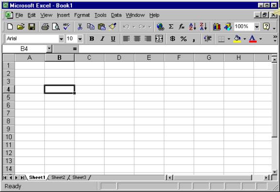
Spreadsheets are very convenient tools when we deal with tables and engineering calculations that can be best performed in the form of tables. In fact a sheet of a spreadsheet is a huge table with the columns being marked by letters, A, B, C,…… etc. and the rows being marked by numbers. It will be helpful if while you are reading this material, you were to activate an excel spreadsheet and look at it from time to time as we learn the various aspects. Here we include the picture of an empty spreadsheet named Book 1.

Note the following :

1) The first three bars at the top of the spreadsheet are the usual menu bars we find in almost all applications. They contain commands for opening, saving, printing files etc.; commands for choosing an appropriate format and font; commands for inserting charts, cutting, pasting etc.

In your spreadsheet window, click on some of these buttons and view the drop menus.

2) There are some special menu buttons of images such as the button Data in the first bar. We will see that this button contains the commands for ordering tables according to our preferences. Another special icon in the second bar is f _x , which can be also activated from the insert button. This is the way to introduce the powerful library functions of spreadsheets, which can perform various complicated calculations.

In your spreadsheet window, click on f_x and view the names of the various functions available. They are classified in various ways, concentrate on the Math functions. Notice that the dialog box gives you a brief description of each function you select.

3) In the fifth line from top there are two white windows. One of them has B4 in it. This is the indication of the current spreadsheet cell. You can see that the column B and the row 4 has been selected thus selecting a particular cell outlined by the thick black line. The other white window depicts the contents of the selected cell.

Enter your last name in a cell you select and watch the contents by looking at both the cell and at the cell content window.

4) At the very bottom of the spreadsheet there are three ( by default) buttons that select different sheets of the same spreadsheet. The number (and also the names ) of these buttons can be changed to whatever we want.

Try selecting other sheets (put different content to a given cell of each sheet) and also try to see if you can change the name of the sheet (double click on the default name).

USING FORMULAS; CELLS AS MEMORY LOCATIONS:

The cells of a spreadsheet may contain characters or labels as they are called. If we enter something which starts with a letter, or anything preceded by the quote symbol ( ' ), then it is treated as a label. The cells may also contain data. If we enter something which starts with a number or with the symbols +, -, = then it is treated like data. The cells can also contain a formula. A formula is an arithmetic expression which contains the arithmetic operators ( +, -, *, /, ^) , some constants and some variables. The variables are entered by the location of the cell which contains the variable. Library functions can also be used to create more complex arithmetic expressions. A formula must always start with the = sign.

Look at the following picture:

Cell A4 contains a label (left justified by default). Cells B2 and C2 contain labels (centered by choice). Cell B4 contains data( the number 3.4) and cell C4 contains a formula. Note that the cell itself displays the value of the formula while the content window displays the formula as entered. This formula calculates the square of the number in cell B4 increased by 5. Note the equal sign in front of the formula.

Try to duplicate the above picture in your own spreadsheet and also try to enter in cell E4 another formula which calculates the value of the polynomial 3 x⁴ + 5.6 x³-3 x + 1.5 , where the value of x is the one contained in cell B4

GENERATING A TABLE BY COPYING A SINGLE FORMULA:

Suppose that we wanted to create a table which listed the values of x ² + 5 versus x as x took values from 3.4 to 4.4 at increments of 0.2. We have the labels ( x and y ) of this table and the first line. How can we create the rest of it?

First we would like to enter the values of x ( 3.6, 3.8, 4.0, 4.2, 4.4) in the cells B5..B9. Please note that the two periods between B5 and B9 denote the range of cells.

The cell B4 contains 3.4, go to cell B5 and enter 3.6, then select both cells B4 and B5 and move your cursor to the lower right corner of the selection box where there is a dark square, as shown in the picture. The cursor should change into a dark cross.

click and drag your mouse down so that the selection box becomes B4..B9. Then release the mouse. The pattern you established in the first two cells will be expanded to the entire range. Now select the cell C4, which contains the formula, copy it and paste it to the entire range C5..C9. You will see the following table generated:

Note that when we copied the formula, the variable of the formula was automatically changed so that each line referred to the appropriate x. In other words, the formula in cell C5 is = 5 + B5 ^ 2, and the one in C6 is = 5 + B6 ^ 2, etc. Check this on your own by selecting various cells in column C.

To familiarize yourselves with the software, try several variations of copying formulas. For example try to copy two cells simultaneously into two columns. Another issue useful in building tables is the selective "freezing" of certain cells as we copy. For example consider that you want to build a table of y = a * x + b versus x, and you would like to store the values of the parameters a and b in the cells A1 and B1. Now, suppose we enter the first line of the table in cells B4 and C4. The formula in C4 must be written as:

= $A$1 * B4 + $B$1

The $ signs ensure that during copying, A1 and B1 will be kept constant without changing to other irrelevant cells.