Numerical
Integration
Consider the following picture which illustrates the graph of a function y = f(x) and two lines parallel to the y axis.
In many engineering applications we have to calculate the area which is bounded
by the curve of the function, the x axis and the two lines x = a and x =
b. Depending on how complex the graph
of the function is this problem may be very easy or very difficult. Consider for example that the picture above
is replaced by:
In calculus we use the symbol of integration ( a large S for sum) to name the
area. We write:
How do we actually perform the evaluation of the "integral"? There are two basic approaches for the calculation
Following the definition of the definite integral, we break the area under the curve into a number of small regular geometric shapes, calculate the sum of the smaller areas and then try to converge to a number which is more or less independent of the particular way we choose to partition the area. This is, in fact, the approach used in numerical integration. Depending on the shapes used, we have a different name.
- When we use rectangles ( we can choose the ones that overestimate, or the ones that underestimate the area) then we talk about Riemann Sums. This method is very important for theoretical considerations but it tends to be inaccurate for actual numerical calculations.
- When we use trapezoids, the method is called trapezoidal. This is the one we want you to learn very well in this course.
- When we use more involved shapes that resemble trapezoids with one of the sides being actually a curve, then we have the family of Simpson's rules.
Note:
When the area of a shape is in the negative side of the y axis (i.e. below the
x axis) then we consider it as a "negative" area, which is supposed
to be subtracted from the sum of the positive areas.
The other approach utilizes the Fundamental Theorem of Calculus to convert the problem of area calculation to a problem of finding the anti derivative of the function in the integral sign, which is called integrand. This is an important analytical tool that you will study very well in the second course of your calculus sequence.
Trapezoidal rule:
Consider the following picture:
The blue curve, which represents the curve y = f(x), bounds an area together with the lines x = x1, x = x4 and the x axis. This area is broken down to three smaller areas, each of which is a trapezoid. The areas of these trapezoids can be calculated easily using the formulas
A1 = 0.5 * [ f(x1) + f(x2) ] * ( x2 - x1)
A2 = 0.5 * [ f(x2) + f(x3) ] * ( x3 - x2)
A1 = 0.5 * [ f(x3) + f(x4) ] * ( x4 - x3)
We can then add all three areas and obtain an estimate for the integral of f(x) from x1 to x4.
We would like to bring your attention to the following points:
The formulas above represent the "area of a trapezoid" formula you learn in elementary geometry classes. For example in the first formula, f(x1) represents the short basis, f(x2) represents the long basis and the difference x2-x1 represents the "height" of the trapezoid. Hence we have "the average base times the height". Equivalently you can think of dividing each trapezoid into two triangles using a diagonal line ( red line shown). Then the formula represents the sum of the areas of two triangles that have different bases but they share the same height x2-x1.
In this example the points x1, x2, x3, and x4 are NOT equidistant. This may be the case in many applications since we may have no control over the location of places where the function value is known.
If however, the points x1, x2, x3, …. are equidistant then
we can write h = ( b - a ) / N , where
a is the lower bound of the integral, b is the upper bound and N is the
number of panels we intend to use in our calculation. Thus for the above example, which uses three panels we would have
h = ( x4 - x1) / 3.
If that was the case ( equidistant x's ), then we could
rewrite the above three formulas as:
A1 = 0.5 [ f( x1) + f( x1 + h ) ] h
A2 = 0.5 [ f( x1+h ) + f( x1 + 2h ) ] h
A1 = 0.5 [ f( x1 + 2h ) + f(x1 + 3h) ] h
We could then combine all three of them and obtain:
Total area = 0.5 h [ f(x1) + 2 f(x1 + h) + 2 f(x1 + 2h) + f(x1 + 3h) ].
This is an alternative form of the trapezoidal rule. It can be stated as follows: The product of 0.5 times h times the sum of the values of the function taken twice at the interior points but once at the first point and at the last.
In general as the number of panels increases and the difference in x's ( the h ) decreases, the accuracy of our calculation increases. We can see this qualitatively since the polygonal line created by the trapezoids approximates the curve better as the number of panels increases.
The calculations needed for the trapezoidal rule can be done in the form of a table where the first column gives the values of the independent variable at the points considered, the second column gives the values of the function at the corresponding points, and the third column gives the individual areas. The sum of the numbers in the third column would then produce the value of the integral. Needless to say that spreadsheets are very handy for this type of calculation.
The following example illustrates the use of this tabular approach.
Simpson's Rule:
Now that we have an understanding of the geometrical approach in approximating integrals, we can try to generalize these ideas using some analysis. Note that if the integrand happened to be a constant function, then the Riemann sum would produce exactly the correct answer for any size h. Similarly if the integrand happened to be a linear function ( a x + b) then the trapezoidal approximation would produce the "exact" answer, again for any size h. Is there a formula that would produce the exact answer for an integrand that happened to be a second order polynomial? The answer to the question is YES and the formula is Simpson's one-third rule. The rule is given for a double panel with partition points a, a+h and a+2h and it is:
The above formula happens to be "exact" even when the integrand is a third order polynomial. This fact makes Simpson's rule very popular. It gives you "more for your money".
The derivation of the above formula is done by considering all possible combinations (linear) of the three values of the function, f(a), f(a+h), and f(a+2h). This gives something like this:
A f(a) + B f(a+h) + C f(a+2h).
We then choose A, B, C so that the formula is exact for f(x) = 1, f(x) = x-a, and f(x) = (x-a)2 . The algebra involved is not bad. You may want to try it on your own. But you must know how to use the Fundamental Theorem of Calculus and obtain that
Generalizing this type of derivation we can obtain other
Simpson's formulas as well as more sophisticated schemes like Gauss
Quadrature.
Romberg Algorithm:
This is a very interesting procedure, which utilizes progressively better trapezoidal approximations to obtain significantly better results than all of them. The best way to explain it is by showing you the table in the following spreadsheet:
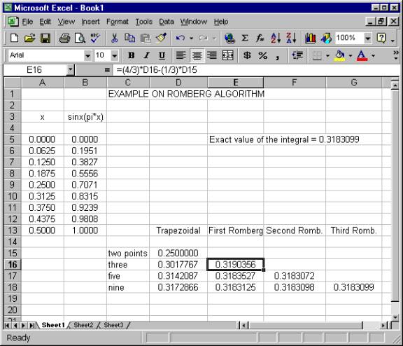
We are calculating the integral of sin(PI * x) from x = 0 to x = 0.5. The "exact" value of this integral is 1/PI or 0.3183099.
The table on the left gives the values of the integrand at the points:
0 & 0.5
0.25
0.125 & 0.3750
0.0625, 0.1875, 0.3125, & 0.4375
The first column of the table on the right ( the column marked as Trapezoidal) gives the approximations to the integral taking progressively more points. Cell D15 gives the approximation using only the end points 0.0 and 1.0. The next cell, D16, gives the approximation using three points. The two end points and the one in the middle , 0.25 . Cell D17 gives the approximation using the above three points plus the two extra ones 0.125 & 0.375 ( placed at the 1/4 of the interval). Finally cell D18 gives the approximation using all of the points, including the ones placed at the 1/8 points of the interval. The picture below illustrates the points used at each approximation:
Now let's look at the First Romberg column of numbers in the table on the right. Cell E16 is calculated from cells D15 and D16 using the formula indicated in the content box of the spreadsheet. The formula is E16 = 4/3 D16 - 1/3 D15. The same formula ( shifted downwards) is used to calculate E17 and E18 . For the Second Romberg column we use similar formulas to calculate cells in column F from cells in column E but the numbers are now 16/15 and 1/15 instead of the 4/3 and 1/3. Finally for the Third Romberg approximation, cell G18, we have the same formula using cells of column F but with numbers 65/64 and 1/64.
It is very clear that the Romberg approximations produce
much better results than the trapezoidal rule alone. It is also important to understand that this improvement is
achieved not by new information about the function but rather by a
"cheap" manipulation of the erroneous data already available. This is possible because the behavior of the
error in the trapezoidal rule is well understood. It is also possible, because
the various data obtained by the trapezoidal rule is generated by strategically
located points as indicated in the picture above. The same idea when
generalized beyond and above integration, caries the name of Richardson
extrapolation.